


Hello, guys! It’s me! Warotan!
So…Who are you?→ABOUT MEJ
This time, I wrote about the important point when plotting and fitting the data with gnuplot.
Please read this if you are a student or a member of society.
Japanese version.
I have written articles about gnulot.
This time, I would like to introduce how to install it in connection with that.
I write similar articles and will add contents, so please read more other articles.
Please note that installation is at your own risk.
How to use gnuplot
gnuplot is a free and popular plotting tool.
Start gnuplot
Enter the following command to start gnuplot.
When gnuplot starts up, it waits for key-in.
For example, please enter this!
It plots the sin curve, right?
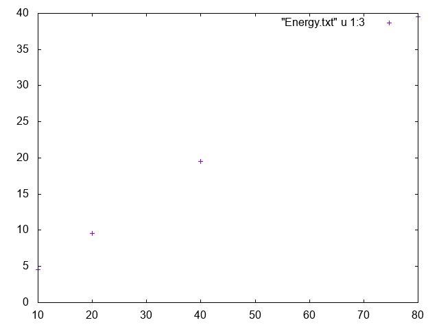
Here, let us use this data.
Please download this and enter this command,
and get this.
By the way, you can get this image in the png format by
set output “foo.png” [Enter]
rep [Enter]
If you would like to know more, please read this article. (English version coming soon, sorry)
Next, we will fit the data with a linear function,
fit f(x) “Energy.txt” u 1:3 via a [Enter]
You will see a lot of fitting results, but ignore them for the moment and type
Then, you will get a linearly fitted graph
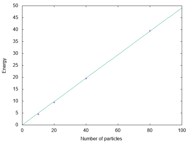
The axis labels are set as
set ylabel “Energy” [Enter]
rep [Enter]
As a side note, \(a = 0.49…\) shows the slope of the fitted function.
Reuse the fitted results
If you quit the gnuplot, then the fitting results will vanish.
There is “fit.log”, but this cannot reproduce the fitting.
So, by executing the following command and save the fitting results,
The extension was set to .fit for now.
You can reuse the results by only loading this .fit file and don’t have to fit it again.
To load this,
However, as a caveat, you have to define the function \(f\left(x\right)\) with the parameter \(a\),
f(x)=a*x [Enter]
plot “Energy.txt” u 1:3,f(x) [Enter]
You will get the same image above.
In fact, you can use a script file .plt with the whole sequence of commands, but I will leave it for the next time because the article becomes so long.
Points to note when reusing
The function to fit should be redefined as it reload only the parameters
I wrote this above, but only the names and values of the parameters will be load, so you should redefine the function.
In the above example, you can save the parameter \(a\) and the value but not the function \(f\).
You can save the fitting results just before the save command
This is a sobering point to keep in mind.
For examle, we just had a fit with function \(f\left(x\right) = ax\), and immediately after that we had another fit with function \(g\left(x\right) = bx^{2}\), like this.
fit g(x) “Energy.txt” u 1:3 via b [Enter]
save fit “Energy_sq.fit” [Enter]
Then, you can save only the results of \(g\left(x\right)\).
So, it is good to save the fitting results to separate files.
Summary
Now, that’s all what I wanted to write.
This time, I wrote from the basic usage of gnuplot to a some practical ones.
Thank you for reading and please spread this blog if you like.
If you have any comment, please let me know from the e-mail address below or the CONTACT on the menu bar.
tsunetthi(at)gmail.com
Please change (at) to @.
Or you can also contact me via twitter (@warotan3)